SummaryPlot#
SummaryPlot takes a DataFrame and shows how its rows are distributed across regions as a stacked bar, using one of two configuration paths:
set_regions()— bin one continuous model-output column against fixed thresholds (e.g. PMV thresholds at -0.5/0.5). You compute the output first (e.g., withpmv_ppd_isoorutci) and store it in the DataFrame.set_categories()— summarize an already-classified per-row category array, for models whose classification cannot be reduced to a single threshold column (see section 11).
This makes it a natural companion to ThresholdPlot: the threshold chart shows where in the input space conditions fall, and the summary bar shows how often they did.
import matplotlib.pyplot as plt
import pandas as pd

from pythermalcomfort.models import pmv_ppd_iso, utci
from pythermalcomfort.plots.matplotlib import SummaryPlot, ThresholdPlot
1. Preparing a Measured Dataset#
Start by computing the model output and storing it in the DataFrame. SummaryPlot only reads the output column — the other columns are ignored.
df = pd.DataFrame(
    {
        "tdb": [20.0, 22.0, 23.5, 24.5, 26.0, 27.5, 29.0, 20.0],
        "rh": [50.0, 45.0, 50.0, 50.0, 55.0, 60.0, 60.0, 65.0],
        "tr": [20.0, 21.5, 23.5, 24.5, 26.0, 28.0, 29.5, 20.0],
        "vr": [0.10, 0.10, 0.10, 0.10, 0.10, 0.10, 0.10, 0.10],
        "met": [1.2, 1.2, 1.2, 1.2, 1.2, 1.2, 1.2, 1.2],
        "clo": [0.90, 0.80, 0.60, 0.50, 0.50, 0.40, 0.35, 0.80],
        "wme": [0.0, 0.0, 0.0, 0.0, 0.0, 0.0, 0.0, 0.0],
    }
)

df["pmv"] = pmv_ppd_iso(
    tdb=df["tdb"],
    tr=df["tr"],
    vr=df["vr"],
    rh=df["rh"],
    met=df["met"],
    clo=df["clo"],
    wme=df["wme"],
).pmv

df.head(4)
| tdb | rh | tr | vr | met | clo | wme | pmv | |
|---|---|---|---|---|---|---|---|---|
| 0 | 20.0 | 50.0 | 20.0 | 0.1 | 1.2 | 0.9 | 0.0 | -0.50 |
| 1 | 22.0 | 45.0 | 21.5 | 0.1 | 1.2 | 0.8 | 0.0 | -0.28 |
| 2 | 23.5 | 50.0 | 23.5 | 0.1 | 1.2 | 0.6 | 0.0 | -0.16 |
| 3 | 24.5 | 50.0 | 24.5 | 0.1 | 1.2 | 0.5 | 0.0 | -0.06 |
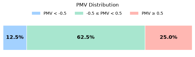
2. Horizontal Bar (Default)#
The default layout is a compact horizontal stacked bar. Each segment shows the share of measurements that fell in that region. Percentage labels appear inside segments that are wide enough to fit them; narrow segments are left unlabelled.
result = (
    SummaryPlot(df)
    .set_regions(output="pmv", thresholds=[-0.5, 0.5])
    .plot(title="PMV Distribution")
)
plt.show()
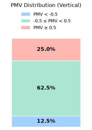
3. Vertical Bar#
Pass vertical=True when the chart needs to fit into a narrow column — for example when placed next to a ThresholdPlot (see section 8). The vertical layout keeps the same compact margins while preserving room for the percentage labels.
result_v = (
    SummaryPlot(df)
    .set_regions(output="pmv", thresholds=[-0.5, 0.5])
    .plot(vertical=True, title="PMV Distribution (Vertical)")
)
plt.show()
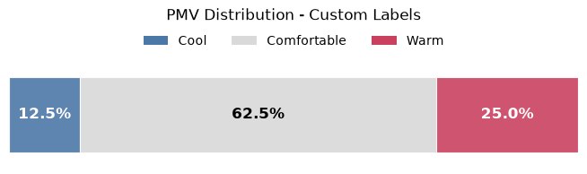
4. Custom Labels, Colors, and Bar Styling#
Pass labels and colors to set_regions to override the auto-generated names and the default palette. Both lists must have length len(thresholds) + 1. Use bar_kws in plot for Matplotlib bar styling such as alpha, linewidth, hatch, or zorder.
result_custom = (
    SummaryPlot(df)
    .set_regions(
        output="pmv",
        thresholds=[-0.5, 0.5],
        labels=["Cool", "Comfortable", "Warm"],
        colors=["#4c78a8", "#d9d9d9", "#c9415f"],
    )
    .plot(
        title="PMV Distribution - Custom Labels",
        bar_kws={"alpha": 0.9, "linewidth": 0.8},
    )
)
plt.show()
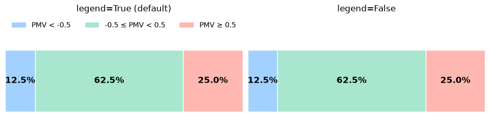
5. Hiding the Legend#
Set legend=False to remove the colour key. When region labels are provided, they are drawn near the bar segments. Pass labels=[] to suppress both the legend and those region labels, which is useful when comparing against a neighbouring plot that already carries the colour key.
fig, (ax0, ax1) = plt.subplots(1, 2, figsize=(9.5, 2.4), constrained_layout=True)

left = (
    SummaryPlot(df)
    .set_regions(output="pmv", thresholds=[-0.5, 0.5])
    .plot(ax=ax0, title="legend=True (default)")
)

right = (
    SummaryPlot(df)
    .set_regions(output="pmv", thresholds=[-0.5, 0.5], labels=[])
    .plot(ax=ax1, title="legend=False", legend=False)
)

right.ax.set_ylim(left.ax.get_ylim())
right.ax.set_title(right.ax.get_title(), y=left.ax.title.get_position()[1])

plt.show()
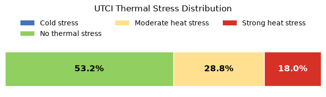
6. UTCI with Official Thermal Stress Labels#
SummaryPlot works with any numeric output column. Here UTCI values are classified into three regions using the official UTCI thermal stress scale. A larger dataset is generated to make the distribution more meaningful.
import numpy as np

rng = np.random.default_rng(7)
n = 120
df_utci = pd.DataFrame(
    {
        "tdb": rng.uniform(10, 38, n),
        "tr": rng.uniform(10, 42, n),
        "v": rng.uniform(0.2, 3.5, n),
        "rh": rng.uniform(20, 80, n),
    }
)
df_utci["utci"] = [
    utci(tdb=r.tdb, tr=r.tr, v=r.v, rh=r.rh).utci
    for r in df_utci.itertuples(index=False)
]
# Drop rows where UTCI is NaN — conditions outside the model's applicability
# limits. SummaryPlot requires all values in the output column to be finite.
df_utci = df_utci.dropna(subset=["utci"])

result_utci = (
    SummaryPlot(df_utci)
    .set_regions(
        output="utci",
        thresholds=[9, 26, 32],
        labels=[
            "Cold stress",
            "No thermal stress",
            "Moderate heat stress",
            "Strong heat stress",
        ],
        colors=["#4575b4", "#91cf60", "#fee090", "#d73027"],
    )
    .plot(title="UTCI Thermal Stress Distribution")
)
plt.show()
/home/docs/checkouts/readthedocs.org/user_builds/pythermalcomfort/envs/latest/lib/python3.13/site-packages/pythermalcomfort/models/utci.py:119: UserWarning: 'v' has value 0.46905381899849224 outside the applicability limits [0.5, 17.0] and will be set to NaN.
  v_valid = valid_range(v, (0.5, 17.0))
/home/docs/checkouts/readthedocs.org/user_builds/pythermalcomfort/envs/latest/lib/python3.13/site-packages/pythermalcomfort/models/utci.py:119: UserWarning: 'v' has value 0.4559036887583093 outside the applicability limits [0.5, 17.0] and will be set to NaN.
  v_valid = valid_range(v, (0.5, 17.0))
/home/docs/checkouts/readthedocs.org/user_builds/pythermalcomfort/envs/latest/lib/python3.13/site-packages/pythermalcomfort/models/utci.py:119: UserWarning: 'v' has value 0.46816562668276857 outside the applicability limits [0.5, 17.0] and will be set to NaN.
  v_valid = valid_range(v, (0.5, 17.0))
/home/docs/checkouts/readthedocs.org/user_builds/pythermalcomfort/envs/latest/lib/python3.13/site-packages/pythermalcomfort/models/utci.py:119: UserWarning: 'v' has value 0.41189960054814195 outside the applicability limits [0.5, 17.0] and will be set to NaN.
  v_valid = valid_range(v, (0.5, 17.0))
/home/docs/checkouts/readthedocs.org/user_builds/pythermalcomfort/envs/latest/lib/python3.13/site-packages/pythermalcomfort/models/utci.py:119: UserWarning: 'v' has value 0.31001947586711376 outside the applicability limits [0.5, 17.0] and will be set to NaN.
  v_valid = valid_range(v, (0.5, 17.0))
/home/docs/checkouts/readthedocs.org/user_builds/pythermalcomfort/envs/latest/lib/python3.13/site-packages/pythermalcomfort/models/utci.py:119: UserWarning: 'v' has value 0.42309163340440015 outside the applicability limits [0.5, 17.0] and will be set to NaN.
  v_valid = valid_range(v, (0.5, 17.0))
/home/docs/checkouts/readthedocs.org/user_builds/pythermalcomfort/envs/latest/lib/python3.13/site-packages/pythermalcomfort/models/utci.py:119: UserWarning: 'v' has value 0.3074424779291368 outside the applicability limits [0.5, 17.0] and will be set to NaN.
  v_valid = valid_range(v, (0.5, 17.0))
/home/docs/checkouts/readthedocs.org/user_builds/pythermalcomfort/envs/latest/lib/python3.13/site-packages/pythermalcomfort/models/utci.py:119: UserWarning: 'v' has value 0.3873553958966254 outside the applicability limits [0.5, 17.0] and will be set to NaN.
  v_valid = valid_range(v, (0.5, 17.0))
/home/docs/checkouts/readthedocs.org/user_builds/pythermalcomfort/envs/latest/lib/python3.13/site-packages/pythermalcomfort/models/utci.py:119: UserWarning: 'v' has value 0.3089789513969277 outside the applicability limits [0.5, 17.0] and will be set to NaN.
  v_valid = valid_range(v, (0.5, 17.0))
7. Reading result.percentages#
result.percentages is a pandas Series indexed by region label. Use it to report compliance figures or pass values to other analyses.
print(result_utci.percentages)
print()

# Pick out a specific region
no_stress = result_utci.percentages["No thermal stress"]
print(f"Time with no thermal stress: {no_stress:.1f} %")

# Check compliance threshold
comfort_share = result_utci.percentages[["No thermal stress"]].sum()
print(f"Overall comfort compliance: {comfort_share:.1f} %")
Cold stress              0.0
No thermal stress       53.2
Moderate heat stress    28.8
Strong heat stress      18.0
Name: proportion, dtype: float64

Time with no thermal stress: 53.2 %
Overall comfort compliance: 53.2 %
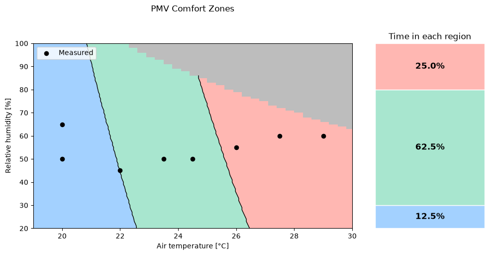
8. Combined View: Comfort Zones + Time Distribution#
Placing a ThresholdPlot and a SummaryPlot side by side answers two questions at once: where in the parameter space do conditions fall, and what fraction of measurements landed in each region. Use labels=[] and legend=False on the SummaryPlot when the neighbouring plot already carries the region legend.
fig, (ax0, ax1) = plt.subplots(
    1,
    2,
    figsize=(10, 5),
    constrained_layout=True,
    gridspec_kw={"width_ratios": [2.8, 1.2]},
)

tp = (
    ThresholdPlot(pmv_ppd_iso)
    .set_x_axis("tdb", 19.0, 30.0, resolution=0.3)
    .set_y_axis("rh", 20.0, 100.0, resolution=1.0)
    .set_params(vr=0.10, met=1.2, clo=0.65, wme=0.0)
    .set_regions(output="pmv", thresholds=[-0.5, 0.5])
    .plot(ax=ax0, title="PMV Comfort Zones", legend_kws={"ncol": 3})
)
tp.ax.scatter(df["tdb"], df["rh"], color="black", s=35, zorder=5, label="Measured")
tp.ax.legend(loc="upper left")
tp.ax.set_xlabel("Air temperature [°C]")
tp.ax.set_ylabel("Relative humidity [%]")

(
    SummaryPlot(df)
    .set_regions(output="pmv", thresholds=[-0.5, 0.5], labels=[])
    .plot(ax=ax1, vertical=True, title="Time in each region", legend=False)
)

plt.show()
/home/docs/checkouts/readthedocs.org/user_builds/pythermalcomfort/envs/latest/lib/python3.13/site-packages/pythermalcomfort/models/pmv_ppd_iso.py:186: UserWarning: 'pa' has 549 values [2715.769018982015, 2726.7018455815864, 2758.2029099036095, 2721.2675656870533, 2768.65110474438, 2800.6368008252034, 2715.1142011436923, 2762.4988924398876, 2810.6003639071737, 2843.0706917467974, 2708.264744475691, 2755.638293698076, 2803.7302191927215, 2852.5496230699673, 2885.5045826683913, 2700.7417437247364, 2748.0921671885685, 2796.1623862524593, 2844.961545945556, 2894.498882232761, 2927.9384735899853, 2739.8829284163994, 2787.9195899014467, 2836.686478806843, 2886.1928726983897, 2936.4481413955546, 2970.3723645115792, 2731.032555687712, 2779.024113108062, 2827.7470126143244, 2877.2105713612264, 2927.424199451224, 2978.397400558348, 3012.806255433173, 2721.5625960241828, 2769.497802950919, 2818.165297799725, 2867.574435327202, 2917.73466391561, 2968.6555262040583, 3020.3466597211423, 3055.240146354767, 2711.494171026181, 2759.3620765245187, 2807.9630502141263, 2857.3064824913877, 2907.40185804008, 2958.2587564699934, 3009.886852956892, 3062.295918883936, 3097.674037276361, 2700.847982684869, 2748.637926793663, 2797.1615570248546, 2846.4282974773337, 2896.4476671830507, 2947.2292807529575, 2998.7828490243764, 3051.1181797097265, 3104.2451780467295, 3140.107928197955, 2737.345928396827, 2785.781682561145, 2834.9610375251905, 2884.8935447405406, 2935.5888518747133, 2987.0567034658357, 3039.30694157876, 3092.3495064625604, 3146.194437209523, 3182.541819119549, 2725.506243398712, 2773.8438741087843, 2822.925438328627, 2872.7605180255264, 2923.358792003748, 2974.7300365663764, 3026.8841261787134, 3079.8310341331435, 3133.5808332153947, 3188.1436963723168, 3224.975710041143, 2713.1386269919713, 2761.368167653958, 2810.341819820742, 2860.0691940961087, 2910.5599985258623, 2961.824039266955, 3013.8712212580394, 3066.711548891591, 3120.355126687527, 3174.812159968229, 3230.0929555351104, 3267.409600962737, 2700.262433148441, 2748.374193576283, 2797.2300919092045, 2846.8397655327, 2897.212949863591, 2948.359479026198, 3000.2892865301624, 3053.012405949702, 3106.5389716044688, 3160.8792192419105, 3216.043486721063, 3272.042214697904, 3309.843491884331, 2734.8811822913694, 2783.609760160594, 2833.0920161644503, 2883.3377112446574, 2934.3567056310726, 2986.1589595265336, 3038.75453379337, 3092.153590641365, 3146.366394317347, 3201.403311796294, 3257.274813473897, 3313.9914738606976, 3352.2773828059253, 2720.907969842985, 2769.499931434298, 2818.8453267449054, 2868.9539404196967, 2919.835656956615, 2971.5004613985548, 3023.9584400268695, 3077.2197810565767, 3131.2947753330277, 3186.1938170302246, 3241.9274043506775, 3298.506140226731, 3355.9407330234912, 3394.7112737275193, 2706.473003444924, 2754.9193194660224, 2804.118680577227, 2854.0808933292165, 2904.815864674943, 2956.333602668573, 3008.6442171660365, 3061.7579205272054, 3115.685028319784, 3170.4359600246908, 3226.0212397431023, 3282.451496905061, 3339.7374669795654, 3397.889992186285, 3437.145164649113, 2739.886250401034, 2788.93066908906, 2838.737429720156, 2889.316459913528, 2940.6777889301893, 2992.8315483805304, 3045.7879729335186, 3099.5574010275413, 3154.150275582991, 3209.5771447163534, 3265.84866245598, 3322.9755894594446, 3380.9687937323997, 3439.8392513490785, 3479.579055570707, 2724.4186682775053, 2773.299497357144, 2822.942018712097, 2873.3561788630846, 2924.552026497839, 2976.539713185435, 3029.3294940924884, 3082.9317287010003, 3137.3568815278772, 3192.6155228461985, 3248.7183294080164, 3305.6760851688578, 3363.499682013828, 3422.2001204852336, 3481.788510511872, 3522.012946492301, 2708.53414045985, 2757.2429895820537, 2806.7127443132545, 2856.953368335134, 2907.974928006013, 2959.7875930821506, 3012.4016374406815, 3065.827439804446, 3120.0754844684825, 3175.156362028213, 3231.0807701094054, 3287.859514099679, 3345.503507881736, 3404.023774568211, 3463.431447238068, 3523.7377696746657, 3564.446837413895, 2740.778594512943, 2790.0673108866017, 2840.1259912693645, 2890.9647179581716, 2942.593677148942, 2995.0231596664617, 3048.263561695928, 3102.3253855164035, 3157.219240235964, 3212.955842528549, 3269.546017372613, 3327.000698791342, 3385.3309305946136, 3444.5478671225947, 3504.6627739909018, 3565.6870288374594, 3606.880728335489, 2723.9233908226993, 2773.023048566037, 2822.89163219115, 2873.5392382254745, 2924.976067581209, 2977.2124262918705, 3030.258726250773, 3084.125485951174, 3138.8233312283614, 3194.362996003446, 3250.755323028885, 3308.01126463582, 3366.1418834830047, 3425.1583533074913, 3485.071959676978, 3545.894100743736, 3607.636288000253, 3649.314619257083, 2706.694092433557, 2755.5969186229636, 2805.26750261913, 2855.715953495698, 2906.952485181585, 2958.987417204246, 3011.831175434799, 3065.4942928350843, 3119.98741020642, 3175.321276940319, 3231.506751770928, 3288.554803529221, 3346.476511899027, 3405.2830681746677, 3464.985776020369, 3525.5960522313617, 3587.1254274965704, 3649.5855471630466, 3691.748510178677, 2737.8055187833684, 2787.2704464232274, 2837.5119566722237, 2888.5402748002466, 2940.365732137695, 2992.9987668272834, 3046.4499245777283, 3100.729859419396, 3155.8493344616663, 3211.8192226522765, 3268.65050753841, 3326.3542840295568, 3384.9417591622346, 3444.4242528663303, 3504.813198733247, 3566.120144785745, 3628.3567542494043, 3691.5348063258402, 3734.182401100271, 2719.6650884956193, 2768.916945133179, 2818.9439742234913, 2869.756410725317, 2921.3645961047946, 2973.778979093805, 3027.0101164503208, 3081.068673720657, 3135.965426003707, 3191.7112587169127, 3248.3171683642345, 3305.794263305892, 3364.1537645298927, 3423.4070064254415, 3483.5654375579934, 3544.640621446125, 3606.6442373401287, 3669.5880810022386, 3733.484065488634, 3776.616292021865, 2701.1915141490285, 2750.223123197817, 2800.02837148299, 2850.617502023755, 2902.0008647784107, 2954.188917409343, 3007.1922260499155, 3061.021466073358, 3115.6874228635857, 3171.2009925880184, 3227.573182972159, 3284.815114076192, 3342.9380190733737, 3401.9532450302286, 3461.872253688649, 3522.7066222496564, 3584.4680441590026, 3647.168329894512, 3710.8194077550725, 3775.4333246514275, 3819.050182943459, 2731.204753195129, 2780.7811579000154, 2831.1397978328014, 2882.291029824019, 2934.245318831504, 2987.0132387138915, 3040.6054730060255, 3095.0328156963956, 3150.3061720065143, 3206.43655917233, 3263.435107227405, 3321.3130597881495, 3380.081774840856, 3439.7527255305645, 3500.337500951856, 3561.847806941319, 3624.2954668718803, 3687.6924224488957, 3752.050734507907, 3817.382583814221, 3861.484073865053, 2711.877260993552, 2761.2179922412292, 2811.339192602213, 2862.251224182612, 2913.9645576242833, 2966.489772884597, 3019.8375600184395, 3074.0187199621355, 3129.0441653194325, 3184.924921149443, 3241.672125756641, 3299.297031482651, 3357.8110055001075, 3417.2255306083375, 3477.5522060309004, 3538.8027482150633, 3600.988991632982, 3664.122889584758, 3728.2165150032793, 3793.282061260741, 3859.3318429770147, 3903.9179647866467, 2741.3541877434823, 2791.2312312873296, 2841.897227304411, 2893.3626505324232, 2945.638085424547, 2998.734226937691, 3052.661881322988, 3107.431966918246, 3163.05551494247, 3219.5436702923716, 3276.9076923409525, 3335.1589557378975, 3394.308951212065, 3454.3692863758197, 3515.351686531236, 3577.2679954782707, 3640.1301763246447, 3703.950312297636, 3768.7406075576628, 3834.513388013575, 3901.2811021398084, 3946.351855708241, 2721.2047172177427, 2770.8311144934123, 2821.24447033343, 2872.4552620066092, 2924.4740768822344, 2977.311613224811, 3030.978680990784, 3085.486202627536, 3140.845213874356, 3197.0668645655073, 3254.1624194353003, 3312.1432589252636, 3371.020879993144, 3430.8068969240226, 3491.5130421433014, 3553.1511670315717, 3615.7332427414776, 3679.2713610163078, 3743.777735010514, 3809.264700112046, 3875.7447147664093, 3943.230361302602, 3988.785746629835, 2700.7842181045635, 2750.1537035711226, 2800.308041243342, 2851.2577093795303, 2903.013296708807, 2955.585503232045, 3008.985141025075, 3063.223135043878, 3118.3105239320844, 3174.258460830466, 3231.0782141885447, 3288.7811685782294, 3347.378825509575, 3406.8828042483897, 3467.3048426359805, 3528.6567979107836, 3590.9506475319076, 3654.198490004685, 3718.4125457079704, 3783.6051577233916, 3849.7887926664293, 3916.9760415192436, 3985.1796204653956, 4031.219637551429, 2729.2135256635593, 2779.102689924503, 2829.784967993272, 2881.2709484256306, 2933.571331411005, 2986.6969295818562, 3040.658668825339, 3095.467589096971, 3151.134845236633, 3207.6717077865765, 3265.089563811582, 3323.399917721158, 3382.614392093886, 3442.744728503636, 3503.802788347938, 3565.8005536782653, 3628.7501280322435, 3692.663737267892, 3757.5537303996334, 3823.4325804362693, 3890.312885220813, 3958.2073682720775, 4027.128879628189, 4073.653528473023, 2708.0247787049393, 2757.6428332225546, 2808.0516762778834, 2859.261894743202, 2911.284187471731, 2964.129366113203, 3017.8083559316674, 3072.332196625603, 3127.712043150065, 3183.959166541181, 3241.0849547426865, 3299.100913434619, 3358.0186668640868, 3417.8499586781977, 3478.6066527588823, 3540.3007340598956, 3602.9443094457474, 3666.5496085325794, 3731.1289845310994, 3796.694915091296, 3863.2600031491475, 3930.8369777751964, 3999.438695024912, 4069.078138790983, 4116.0874193946165, 2735.9425599287015, 2786.07214078155, 2837.0006626312634, 2888.738821493132, 2941.2974265178314, 2994.687400815401, 3048.919782281478, 3104.005724425867, 3159.956497203158, 3216.7834878457293, 3274.4982016987965, 3333.1122630576565, 3392.6374160070154, 3453.085525262509, 3514.4685770141286, 3576.7986797718536, 3640.088065213229, 3704.3490890329153, 3769.5942317943063, 3835.836099782959, 3903.087425862025, 3971.36107032958, 4040.6700217777457, 4111.027397953777, 4158.5213103162105, 2714.0156357217784, 2763.8603411524637, 2814.5014483405453, 2865.9496489846438, 2918.2157482430616, 2971.3106655639317, 3025.245435517599, 3080.0312086312892, 3135.6792522261308, 3192.2009512562518, 3249.6078091502773, 3307.911448654907, 3367.123612680694, 3427.256165149944, 3488.3210918468203, 3550.3305012693745, 3613.296625483811, 3677.2318209807113, 3742.1485695332512, 3808.0594790575137, 3874.9772844746217, 3942.914848574903, 4011.8851628839634, 4081.90134853058, 4152.97665711657, 4200.955201237804, 2741.4299350725037, 2791.778122376226, 2842.9307558995406, 2894.8986353380237, 2947.6926749929917, 3001.323904610032, 3055.803470219797, 3111.1426349811004, 3167.3527800263946, 3224.445405309345, 3282.4321304548257, 3341.324695611017, 3401.1349623037313, 3461.8749142928727, 3523.5566584311314, 3586.192425524621, 3649.794571195769, 3714.375576748193, 3779.948050033587, 3846.524726320721, 3914.1184691662847, 3982.7422712877806, 4052.409255438347, 4123.132675283414, 4194.925916279364, 4243.389092159399] at indices [1709, 1746, 1747, 1783, 1784, 1785, 1820, 1821, 1822, 1823, 1857, 1858, 1859, 1860, 1861, 1894, 1895, 1896, 1897, 1898, 1899, 1932, 1933, 1934, 1935, 1936, 1937, 1969, 1970, 1971, 1972, 1973, 1974, 1975, 2006, 2007, 2008, 2009, 2010, 2011, 2012, 2013, 2043, 2044, 2045, 2046, 2047, 2048, 2049, 2050, 2051, 2080, 2081, 2082, 2083, 2084, 2085, 2086, 2087, 2088, 2089, 2118, 2119, 2120, 2121, 2122, 2123, 2124, 2125, 2126, 2127, 2155, 2156, 2157, 2158, 2159, 2160, 2161, 2162, 2163, 2164, 2165, 2192, 2193, 2194, 2195, 2196, 2197, 2198, 2199, 2200, 2201, 2202, 2203, 2229, 2230, 2231, 2232, 2233, 2234, 2235, 2236, 2237, 2238, 2239, 2240, 2241, 2267, 2268, 2269, 2270, 2271, 2272, 2273, 2274, 2275, 2276, 2277, 2278, 2279, 2304, 2305, 2306, 2307, 2308, 2309, 2310, 2311, 2312, 2313, 2314, 2315, 2316, 2317, 2341, 2342, 2343, 2344, 2345, 2346, 2347, 2348, 2349, 2350, 2351, 2352, 2353, 2354, 2355, 2379, 2380, 2381, 2382, 2383, 2384, 2385, 2386, 2387, 2388, 2389, 2390, 2391, 2392, 2393, 2416, 2417, 2418, 2419, 2420, 2421, 2422, 2423, 2424, 2425, 2426, 2427, 2428, 2429, 2430, 2431, 2453, 2454, 2455, 2456, 2457, 2458, 2459, 2460, 2461, 2462, 2463, 2464, 2465, 2466, 2467, 2468, 2469, 2491, 2492, 2493, 2494, 2495, 2496, 2497, 2498, 2499, 2500, 2501, 2502, 2503, 2504, 2505, 2506, 2507, 2528, 2529, 2530, 2531, 2532, 2533, 2534, 2535, 2536, 2537, 2538, 2539, 2540, 2541, 2542, 2543, 2544, 2545, 2565, 2566, 2567, 2568, 2569, 2570, 2571, 2572, 2573, 2574, 2575, 2576, 2577, 2578, 2579, 2580, 2581, 2582, 2583, 2603, 2604, 2605, 2606, 2607, 2608, 2609, 2610, 2611, 2612, 2613, 2614, 2615, 2616, 2617, 2618, 2619, 2620, 2621, 2640, 2641, 2642, 2643, 2644, 2645, 2646, 2647, 2648, 2649, 2650, 2651, 2652, 2653, 2654, 2655, 2656, 2657, 2658, 2659, 2677, 2678, 2679, 2680, 2681, 2682, 2683, 2684, 2685, 2686, 2687, 2688, 2689, 2690, 2691, 2692, 2693, 2694, 2695, 2696, 2697, 2715, 2716, 2717, 2718, 2719, 2720, 2721, 2722, 2723, 2724, 2725, 2726, 2727, 2728, 2729, 2730, 2731, 2732, 2733, 2734, 2735, 2752, 2753, 2754, 2755, 2756, 2757, 2758, 2759, 2760, 2761, 2762, 2763, 2764, 2765, 2766, 2767, 2768, 2769, 2770, 2771, 2772, 2773, 2790, 2791, 2792, 2793, 2794, 2795, 2796, 2797, 2798, 2799, 2800, 2801, 2802, 2803, 2804, 2805, 2806, 2807, 2808, 2809, 2810, 2811, 2827, 2828, 2829, 2830, 2831, 2832, 2833, 2834, 2835, 2836, 2837, 2838, 2839, 2840, 2841, 2842, 2843, 2844, 2845, 2846, 2847, 2848, 2849, 2864, 2865, 2866, 2867, 2868, 2869, 2870, 2871, 2872, 2873, 2874, 2875, 2876, 2877, 2878, 2879, 2880, 2881, 2882, 2883, 2884, 2885, 2886, 2887, 2902, 2903, 2904, 2905, 2906, 2907, 2908, 2909, 2910, 2911, 2912, 2913, 2914, 2915, 2916, 2917, 2918, 2919, 2920, 2921, 2922, 2923, 2924, 2925, 2939, 2940, 2941, 2942, 2943, 2944, 2945, 2946, 2947, 2948, 2949, 2950, 2951, 2952, 2953, 2954, 2955, 2956, 2957, 2958, 2959, 2960, 2961, 2962, 2963, 2977, 2978, 2979, 2980, 2981, 2982, 2983, 2984, 2985, 2986, 2987, 2988, 2989, 2990, 2991, 2992, 2993, 2994, 2995, 2996, 2997, 2998, 2999, 3000, 3001, 3014, 3015, 3016, 3017, 3018, 3019, 3020, 3021, 3022, 3023, 3024, 3025, 3026, 3027, 3028, 3029, 3030, 3031, 3032, 3033, 3034, 3035, 3036, 3037, 3038, 3039, 3052, 3053, 3054, 3055, 3056, 3057, 3058, 3059, 3060, 3061, 3062, 3063, 3064, 3065, 3066, 3067, 3068, 3069, 3070, 3071, 3072, 3073, 3074, 3075, 3076, 3077] outside the applicability limits [0.0, 2700.0] and will be set to NaN.
  pa_valid = valid_range(pa, (0.0, 2700.0))
/home/docs/checkouts/readthedocs.org/user_builds/pythermalcomfort/envs/latest/lib/python3.13/site-packages/pythermalcomfort/models/pmv_ppd_iso.py:187: UserWarning: 'pmv' has 38 values [2.0087009241331524, 2.0181515189043893, 2.0276021136756257, 2.037052708446862, 2.046503303218099, 2.0559538979893346, 2.0051131861136238, 2.065404492760571, 2.014455846913541, 2.0748550875318075, 2.0237985077134586, 2.0843056823030444, 2.033141168513375, 2.093756277074281, 2.0424838293132925, 2.1032068718455172, 2.0518264901132097, 2.1126574666167537, 2.0611691509131274, 2.1221080613879906, 2.070511811713044, 2.1315586561592266, 2.0798544725129613, 2.141009250930463, 2.089197133312879, 2.1504598457017, 2.0067546706288004, 2.098539794112796, 2.1599104404729363, 2.015937438283585, 2.1078824549127138, 2.169361035244173, 2.02512020593837, 2.117225115712631, 2.1788116300154092, 2.034302973593155, 2.1265677765125486, 2.188262224786646] at indices [2355, 2393, 2431, 2469, 2507, 2545, 2582, 2583, 2620, 2621, 2658, 2659, 2696, 2697, 2734, 2735, 2772, 2773, 2810, 2811, 2848, 2849, 2886, 2887, 2924, 2925, 2961, 2962, 2963, 2999, 3000, 3001, 3037, 3038, 3039, 3075, 3076, 3077] outside the applicability limits [-2, 2] and will be set to NaN.
  pmv_valid = valid_range(pmv, (-2, 2))
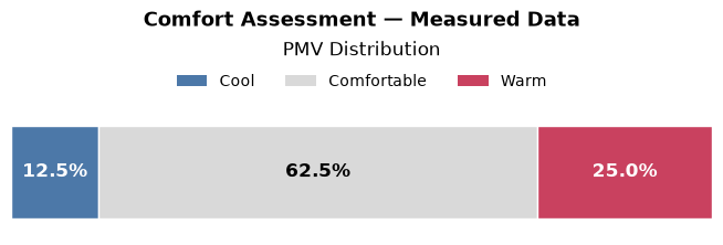
9. Using result.fig#
result.fig is the underlying Figure. Use it for figure-level operations such as adding a super-title or saving to disk.
r = (
    SummaryPlot(df)
    .set_regions(
        output="pmv",
        thresholds=[-0.5, 0.5],
        labels=["Cool", "Comfortable", "Warm"],
        colors=["#4c78a8", "#d9d9d9", "#c9415f"],
    )
    .plot(title="PMV Distribution")
)

r.fig.suptitle(
    "Comfort Assessment — Measured Data", y=1.14, fontsize=13, fontweight="bold"
)

# r.fig.savefig("pmv_summary.png", dpi=150, bbox_inches="tight")
plt.show()
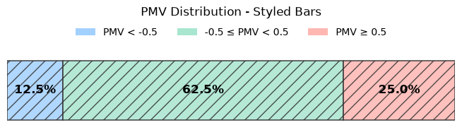
10. Custom Bar Properties with bar_kws#
bar_kws forwards Matplotlib bar keyword arguments to the stacked bar segments. This is useful for changing visual properties such as transparency, edge styling, line width, or hatch patterns.
(
    SummaryPlot(df)
    .set_regions(output="pmv", thresholds=[-0.5, 0.5])
    .plot(
        title="PMV Distribution - Styled Bars",
        bar_kws={
            "alpha": 0.85,
            "edgecolor": "#333333",
            "linewidth": 1.2,
            "hatch": "//",
        },
    )
)

plt.show()
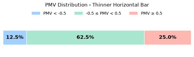
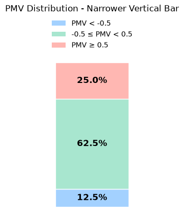
Matplotlib uses different size arguments for horizontal and vertical bars. For a horizontal barh chart, height controls the bar thickness. For a vertical bar chart, width controls the bar thickness.
(
    SummaryPlot(df)
    .set_regions(output="pmv", thresholds=[-0.5, 0.5])
    .plot(
        title="PMV Distribution - Thinner Horizontal Bar",
        bar_kws={"height": 0.42},
    )
)

plt.show()
(
    SummaryPlot(df)
    .set_regions(output="pmv", thresholds=[-0.5, 0.5])
    .plot(
        vertical=True,
        title="PMV Distribution - Narrower Vertical Bar",
        bar_kws={"width": 0.52},
    )
)

plt.show()
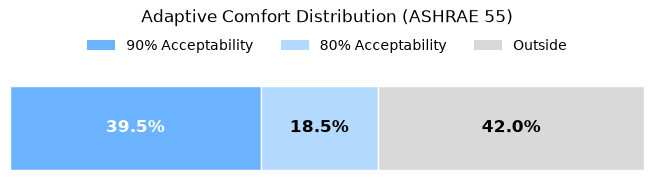
11. Classifying Non-Threshold Model Output (Adaptive Comfort)#
set_regions() bins one continuous output column against fixed thresholds — great for PMV, UTCI, or anything else that reduces to a single number plus cutoffs. Some models don’t fit that shape: adaptive comfort’s acceptability depends on each row’s own running mean temperature, so the model itself returns per-row boolean acceptability fields rather than one column to threshold.
For cases like this, set_categories() takes an already-classified array of per-row category labels — computed however makes sense for the model at hand — and summarizes it the same way set_regions() does. np.select picks the narrowest (best) band each row satisfies, in priority order, falling back to "Outside" for rows that satisfy none:
import numpy as np

from pythermalcomfort.models import adaptive_ashrae

rng = np.random.default_rng(42)
n = 200
df_adaptive = pd.DataFrame(
    {
        "tdb": rng.uniform(15, 35, n),
        "tr": rng.uniform(15, 35, n),
        "t_rm": rng.uniform(10, 33, n),
        "v": 0.2,
    }
)

adaptive_result = adaptive_ashrae(
    tdb=df_adaptive["tdb"],
    tr=df_adaptive["tr"],
    t_running_mean=df_adaptive["t_rm"],
    v=df_adaptive["v"],
)
categories = np.select(
    [adaptive_result.acceptability_90, adaptive_result.acceptability_80],
    ["90% Acceptability", "80% Acceptability"],
    default="Outside",
)

result_adaptive = (
    SummaryPlot(df_adaptive)
    .set_categories(
        categories,
        labels=["90% Acceptability", "80% Acceptability", "Outside"],
        colors=["#6BB3FF", "#B3D9FF", "#D9D9D9"],
    )
    .plot(title="Adaptive Comfort Distribution (ASHRAE 55)")
)
plt.show()