Combined Plot Examples

This notebook shows how to combine different pythermalcomfort.plots.matplotlib chart types with each other and with standard Matplotlib code. These are practical recipes, not API references — see threshold_plot.ipynb, summary_plot.ipynb, adaptive_plot.ipynb, and psychrometric_plot.ipynb for full API coverage.

import matplotlib.pyplot as plt
import numpy as np
import pandas as pd

from pythermalcomfort.models import adaptive_ashrae, pmv_ppd_iso, utci
from pythermalcomfort.plots.matplotlib import AdaptivePlot, SummaryPlot, ThresholdPlot

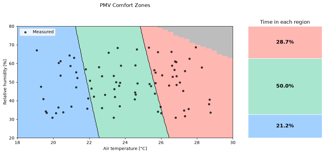
1. Comfort Zone + Measurement Summary

Place a ThresholdPlot and a SummaryPlot side by side to show both where conditions fall within the comfort space and how much time was spent in each region. The two charts share the same region definition, so colours and boundaries match automatically.

# Measured dataset
rng = np.random.default_rng(42)
n = 80
df = pd.DataFrame(
    {
        "tdb": rng.uniform(19, 29, n),
        "rh": rng.uniform(30, 70, n),
        "tr": rng.uniform(19, 30, n),
        "vr": np.full(n, 0.1),
        "met": np.full(n, 1.2),
        "clo": rng.uniform(0.4, 0.9, n),
        "wme": np.zeros(n),
    }
)
df["pmv"] = [
    pmv_ppd_iso(
        tdb=r.tdb, tr=r.tr, vr=r.vr, rh=r.rh, met=r.met, clo=r.clo, wme=r.wme
    ).pmv
    for r in df.itertuples(index=False)
]

thresholds = [-0.5, 0.5]

fig, (ax0, ax1) = plt.subplots(
    1,
    2,
    figsize=(11, 5),
    constrained_layout=True,
    gridspec_kw={"width_ratios": [2.8, 1.2]},
)

# Left: threshold chart with measured points overlaid
tp = (
    ThresholdPlot(pmv_ppd_iso)
    .set_x_axis("tdb", 18.0, 30.0, resolution=0.3)
    .set_y_axis("rh", 20.0, 80.0, resolution=1.0)
    .set_params(vr=0.10, met=1.2, clo=0.65, wme=0.0)
    .set_regions(output="pmv", thresholds=thresholds)
    .plot(ax=ax0, title="PMV Comfort Zones")
)
tp.ax.scatter(
    df["tdb"], df["rh"], color="black", s=18, zorder=5, alpha=0.7, label="Measured"
)
tp.ax.legend(loc="upper left")
tp.ax.set_xlabel("Air temperature [°C]")
tp.ax.set_ylabel("Relative humidity [%]")

# Right: summary bar showing time share per region
(
    SummaryPlot(df)
    .set_regions(output="pmv", thresholds=thresholds, labels=[])
    .plot(ax=ax1, vertical=True, title="Time in each region", legend=False)
)

plt.show()

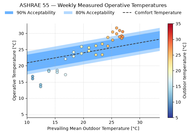
2. Adaptive Chart with Seasonal Measured Data

Plot measured operative temperatures on top of an adaptive comfort chart. Colour the points by outdoor temperature to show seasonal variation.

# Synthetic seasonal dataset (one point per week across a year)
weeks = 52
t_out = 15 + 12 * np.sin(np.linspace(-np.pi / 2, 3 * np.pi / 2, weeks))
t_op = t_out + rng.normal(3.5, 1.5, weeks)

result = (
    AdaptivePlot(adaptive_ashrae)
    .set_params(v=0.2)
    .plot(title="ASHRAE 55 — Weekly Measured Operative Temperatures")
)

sc = result.ax.scatter(
    t_out,
    t_op,
    c=t_out,
    cmap="RdYlBu_r",
    vmin=5,
    vmax=35,
    s=40,
    edgecolors="black",
    linewidths=0.4,
    zorder=5,
)
plt.colorbar(sc, ax=result.ax, label="Outdoor temperature [°C]")
plt.show()

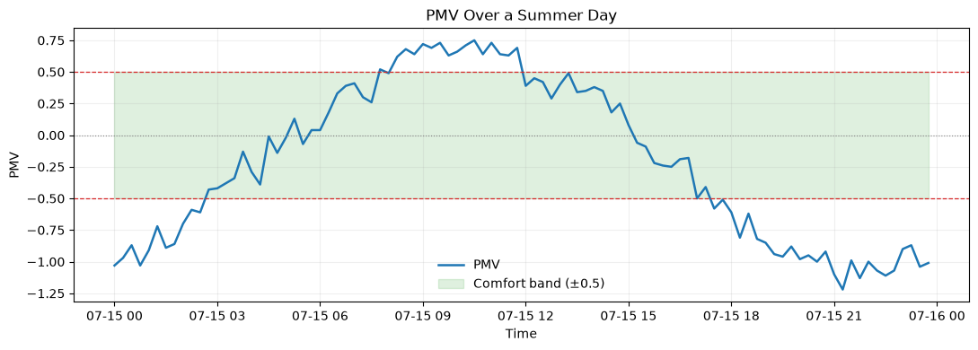
3. PMV Time Series with Comfort Band

Shows how PMV evolves over a day or monitoring period. The shaded band marks the ±0.5 comfort interval.

n = 96
ts = pd.date_range("2026-07-15", periods=n, freq="15min")
tdb = 24 + 3 * np.sin(np.linspace(0, 2 * np.pi, n) - 1.2) + rng.normal(0, 0.3, n)
rh = 52 + 8 * np.sin(np.linspace(0, 2 * np.pi, n) + 0.5) + rng.normal(0, 1.0, n)

pmv_ts = [
    pmv_ppd_iso(tdb=t, tr=t, vr=0.1, rh=r, met=1.2, clo=0.5, wme=0.0).pmv
    for t, r in zip(tdb, rh, strict=False)
]

fig, ax = plt.subplots(figsize=(11, 4))
ax.plot(ts, pmv_ts, lw=1.8, color="#1f77b4", label="PMV")
ax.fill_between(ts, -0.5, 0.5, color="#2ca02c", alpha=0.15, label="Comfort band (±0.5)")
ax.axhline(0.5, color="#d62728", ls="--", lw=0.9)
ax.axhline(-0.5, color="#d62728", ls="--", lw=0.9)
ax.axhline(0.0, color="gray", ls=":", lw=0.8)
ax.set_title("PMV Over a Summer Day")
ax.set_ylabel("PMV")
ax.set_xlabel("Time")
ax.legend(frameon=False)
ax.grid(alpha=0.2)
plt.tight_layout()
plt.show()

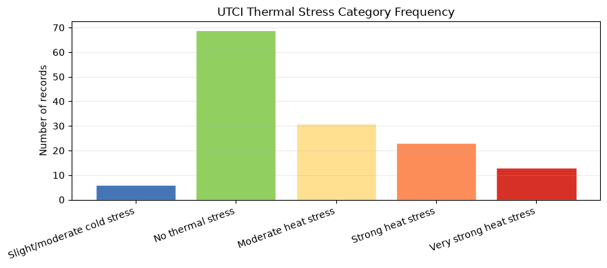
4. UTCI Category Frequency

Classify UTCI values into the official thermal-stress categories and display how often each category occurred in a dataset. Uses pd.cut with the standard UTCI thresholds.

# Synthetic outdoor monitoring dataset
m = 150
tout = pd.DataFrame(
    {
        "tdb": rng.uniform(8, 40, m),
        "tr": rng.uniform(8, 45, m),
        "v": rng.uniform(0.2, 4.0, m),
        "rh": rng.uniform(20, 85, m),
    }
)
tout["utci"] = [
    utci(tdb=r.tdb, tr=r.tr, v=r.v, rh=r.rh).utci for r in tout.itertuples(index=False)
]

bins = [-np.inf, 9, 26, 32, 38, np.inf]
labels = [
    "Slight/moderate cold stress",
    "No thermal stress",
    "Moderate heat stress",
    "Strong heat stress",
    "Very strong heat stress",
]
colors = ["#4575b4", "#91cf60", "#fee090", "#fc8d59", "#d73027"]
tout["category"] = pd.cut(tout["utci"], bins=bins, labels=labels, right=False)
counts = tout["category"].value_counts().reindex(labels, fill_value=0)

fig, ax = plt.subplots(figsize=(9, 4))
ax.bar(counts.index, counts.values, color=colors, edgecolor="white")
ax.set_title("UTCI Thermal Stress Category Frequency")
ax.set_ylabel("Number of records")
ax.grid(axis="y", alpha=0.25)
plt.xticks(rotation=20, ha="right")
plt.tight_layout()
plt.show()

/home/docs/checkouts/readthedocs.org/user_builds/pythermalcomfort/envs/latest/lib/python3.11/site-packages/pythermalcomfort/models/utci.py:119: UserWarning: 'v' has value 0.3716578445598203 outside the applicability limits [0.5, 17.0] and will be set to NaN.
  v_valid = valid_range(v, (0.5, 17.0))
/home/docs/checkouts/readthedocs.org/user_builds/pythermalcomfort/envs/latest/lib/python3.11/site-packages/pythermalcomfort/models/utci.py:119: UserWarning: 'v' has value 0.47292413391096066 outside the applicability limits [0.5, 17.0] and will be set to NaN.
  v_valid = valid_range(v, (0.5, 17.0))
/home/docs/checkouts/readthedocs.org/user_builds/pythermalcomfort/envs/latest/lib/python3.11/site-packages/pythermalcomfort/models/utci.py:118: UserWarning: 'tr - tdb' has value -31.117911792623552 outside the applicability limits [-30.0, 70.0] and will be set to NaN.
  diff_valid = valid_range(tr - tdb, (-30.0, 70.0), param_name="tr - tdb")
/home/docs/checkouts/readthedocs.org/user_builds/pythermalcomfort/envs/latest/lib/python3.11/site-packages/pythermalcomfort/models/utci.py:119: UserWarning: 'v' has value 0.3142073992924794 outside the applicability limits [0.5, 17.0] and will be set to NaN.
  v_valid = valid_range(v, (0.5, 17.0))
/home/docs/checkouts/readthedocs.org/user_builds/pythermalcomfort/envs/latest/lib/python3.11/site-packages/pythermalcomfort/models/utci.py:119: UserWarning: 'v' has value 0.39040542084834834 outside the applicability limits [0.5, 17.0] and will be set to NaN.
  v_valid = valid_range(v, (0.5, 17.0))
/home/docs/checkouts/readthedocs.org/user_builds/pythermalcomfort/envs/latest/lib/python3.11/site-packages/pythermalcomfort/models/utci.py:119: UserWarning: 'v' has value 0.20877333582961963 outside the applicability limits [0.5, 17.0] and will be set to NaN.
  v_valid = valid_range(v, (0.5, 17.0))
/home/docs/checkouts/readthedocs.org/user_builds/pythermalcomfort/envs/latest/lib/python3.11/site-packages/pythermalcomfort/models/utci.py:119: UserWarning: 'v' has value 0.4358398048525899 outside the applicability limits [0.5, 17.0] and will be set to NaN.
  v_valid = valid_range(v, (0.5, 17.0))
/home/docs/checkouts/readthedocs.org/user_builds/pythermalcomfort/envs/latest/lib/python3.11/site-packages/pythermalcomfort/models/utci.py:119: UserWarning: 'v' has value 0.35296421177171033 outside the applicability limits [0.5, 17.0] and will be set to NaN.
  v_valid = valid_range(v, (0.5, 17.0))